Every principle in this series so far has placed something in the flow path: a heated sensor, a restriction, a vibrating tube, a pair of gears.
Ultrasound can take a different route:
The sensors can sit entirely outside the pipe.
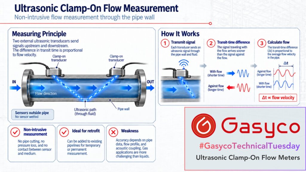
Two transducers are clamped onto the existing pipe. An ultrasonic signal crosses the pipe wall and the medium, and the flow velocity is derived from a difference in transit time. The pipe itself becomes part of the measuring instrument. Since 2023, ISO 24062 has described this method specifically for clamp-on transit-time meters on liquids and gases.
One note on scope. We do not use this technology. Our applications are relatively small flows of pure gases that we want to measure, and above all control, with high accuracy. As this article will show, that is almost exactly the combination in which clamp-on ultrasound is at its weakest.
From Two Transit Times to a Flow Velocity
The dominant principle in industrial clamp-on meters is the transit-time difference method. Two transducers are arranged so that the sound crosses the medium at an angle to the flow. Both act alternately as transmitter and receiver.
With the flow: t↓ = L / (c + v × cos α)
Against the flow: t↑ = L / (c − v × cos α)
L is the acoustic path length, c the speed of sound in the medium, v the flow velocity along the pipe axis and α the angle between sound path and flow.
The signal travelling with the flow arrives slightly earlier, the one against it slightly later. What matters is the tiny difference between them. Modern clamp-on instruments specify timing uncertainties of a few tenths of a nanosecond for a single sensor pair.
There is an elegant detail here. If both transit times are measured, the velocity can be calculated from their reciprocals, v = L / (2 cos α) × (1/t↓ − 1/t↑), and the speed of sound cancels out. The velocity measurement is therefore largely independent of the gas composition. As a by-product, the instrument also obtains the speed of sound itself.
How Does the Sound Get Through the Pipe?
Between transducer and medium lie a coupling layer, the pipe wall and possibly a lining. Even a thin air gap between sensor and metal would reflect most of the acoustic energy, which is why an acoustic couplant is always used.
The sound is refracted at every material boundary, much as light changes direction between air and glass, following Snell’s law. The instrument therefore needs outer diameter, wall thickness, pipe material, any lining, and the speed of sound and temperature of the medium to calculate how far apart the sensors must be mounted.
Z, V and W Arrangements
In a Z arrangement the sensors sit on opposite sides of the pipe and the sound crosses the medium once. That gives the shortest path and the least attenuation, which helps with large diameters and difficult acoustics.
In a V arrangement both sensors sit on the same side and the sound reflects off the opposite wall; in a W arrangement it crosses several times. A longer path increases the time difference, but every reflection weakens the signal.
Why Pipe Geometry Decides Accuracy
The volume flow is calculated from the mean velocity and the cross-section:
Q = v × A, with v the mean velocity and A = π × D² / 4
The inner diameter enters squared: one percent error in the assumed diameter causes roughly two percent error in the flow through the cross-section alone. Wall tolerances, corrosion, deposits or linings change the real geometry, so on existing plants the wall thickness should be measured, not taken from a pipe table.
The obvious advantage of needing no dedicated measuring tube therefore shifts part of the responsibility onto the existing pipe.
Why Clamp-On Is Much Harder on Gas Than on Liquids
The decisive quantity is the acoustic impedance, Z = ρ × c, the product of density and speed of sound. Steel has an acoustic impedance of roughly 45 million, air at atmospheric pressure around 400, in the same units. At normal incidence, well under one ten-thousandth of the acoustic energy crosses a single steel-to-air boundary. And the signal has to cross into the gas and back out again.
At the same time, sound travels directly through the pipe wall to the receiver, and this wall-borne signal can be far stronger than the wave that crossed the gas. Modern gas systems use optimised transducers, signal processing and damping material to separate the two.
Pressure helps: as gas pressure rises, density and therefore acoustic impedance increase. A 2026 study on natural gas found that metal pipes require a minimum internal pressure for reliable measurement, while plastic pipes worked even at atmospheric pressure.
Pipe material, wall thickness, gas type, pressure and diameter decide together whether enough acoustic energy passes through the medium.
The Second Challenge: The Flow Profile
The ultrasound measures the mean velocity along a specific acoustic path, not across the whole cross-section. A profile correction factor bridges the two, and it depends on the Reynolds number. According to a 2025 PTB and Emerson Flexim paper, this factor ranges from about 0.75 for laminar flow to typically 0.90 to 0.97 in turbulent flow, and the transition between the two can extend up to a Reynolds number of around 10,000.
Behind bends, partially closed valves or T-pieces the profile becomes asymmetric or swirling. The same paper notes that uncorrected profile effects can cause errors of up to 15 percent. The 2026 natural gas study measured deviations of up to 9 percent within ten diameters downstream of a single bend, and only reached ±2 percent beyond twenty diameters, twice the distance the manufacturer recommended.
This is the fundamental difference to Coriolis, where the entire mass passing through the tube acts on the measurement. Here, one or a few paths sample a profile.
Volume Flow Is Not Yet Mass Flow
The transit-time method delivers a volume flow at operating conditions. For liquids that is often sufficient. For gases it is not: 10 m³/h at 1 bar absolute contains a tenth of the mass of 10 m³/h at 10 bar. Standard volume or mass flow additionally requires absolute pressure, temperature, gas composition and, at higher pressures, compressibility.
Clamp-On and Inline Ultrasound Are Not the Same Thing
Inline meters with several wetted acoustic paths in a dedicated spool piece, covered by ISO 17089, are an established standard for high-accuracy gas metering, including natural gas custody transfer. They know their own geometry exactly and sample the profile along several paths. Clamp-on trades part of that accuracy for measuring without opening the pipe.
Strengths
- fully non-invasive, no need to open the pipe
- retrofit on existing plants, temporary and comparison measurements
- no pressure drop and no moving parts
- no contact with corrosive or high-purity media
- economically attractive on very large pipe diameters
Weaknesses
- exact pipe geometry must be known
- wall material, coatings and deposits affect sound transmission
- sensor positioning and coupling are part of the measurement quality
- disturbed flow profiles cause substantial errors
- gas is far more demanding than liquid because of its low acoustic impedance
- small velocities produce only very small transit-time differences
- mass or standard volume flow of gases requires additional process values
The greatest advantage of the technology, that the sensor never touches the medium, is also the origin of most of its challenges.
Bonus: What About the Doppler Method?
The Doppler method uses echoes from particles or bubbles moving with the flow; the frequency shift gives the velocity. That suits contaminated liquids and slurries, but clean technical gases offer nothing to reflect the sound. Precise clamp-on measurement on clean media almost always means transit time.
Where Ultrasound Sits in This Series, and Why We Do Not Use It
Every principle in this series has leaned on a different property of the medium. Thermal instruments on heat capacity, laminar flow elements on viscosity, orifices and Venturis on density, critical nozzles on the ratio of specific heats. Coriolis needed none of them.
Clamp-on ultrasound is a curious case. The speed of sound cancels out of the velocity calculation, but viscosity returns through the back door: the profile correction depends on the Reynolds number. And density is needed again to get from volume to mass.
For our applications, several of the effects in this article stack up. Small flows mean small pipes or low velocities, and both shrink the time difference and the signal. Commercial gas clamp-on meters typically start at pipe sizes of around 20 to 50 millimetres. Small flows also mean low Reynolds numbers, exactly the laminar and transitional range where the profile factor swings by around twenty percent. Pure gases at moderate pressure in metal pipes are acoustically the hardest case. And a clamp-on meter measures, but it does not control.
Deviations of around ±2 percent under good conditions, as reported in the 2026 study, are fine for consumption monitoring and on-site verification. They are not what precise gas mixing requires.
Conclusion
Clamp-on ultrasound turns an existing pipe into a measuring point without opening it. The principle itself is elegant: sound travels slightly faster with the flow than against it.
The real challenge lies in everything around that equation. The sound has to get through wall and medium, the geometry has to be known, the profile has to be captured representatively, and with gases a reliable transit time has to be extracted from a very weak signal.
Where those conditions are under control, the method offers what almost no other technology does: flow measurement without a process connection, without pressure drop and without any contact between sensor and medium.