Differential pressure is one of the oldest and most versatile principles in flow measurement. The basic idea is simple:
When a fluid passes through a defined flow resistance or a change in cross-section, a measurable pressure difference appears. That difference can be converted into a flow rate.
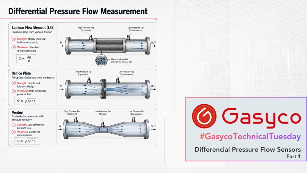
What the name hides is how differently that pressure difference can be created. In a Laminar Flow Element (LFE), viscous friction inside small channels dominates. An orifice plate creates an abrupt acceleration and flow separation. A Venturi accelerates the gas in a controlled way and recovers much of the pressure afterwards.
Three designs, one label, and very different behaviour in practice. This article covers the three subsonic variants. Part two deals with what happens when a gas is accelerated so far that the speed of sound comes into play.
Before we measure: laminar or turbulent?
In a laminar flow the fluid moves in orderly parallel layers, and the viscosity of the fluid strongly determines its behaviour. In a turbulent flow, eddies and velocity fluctuations appear, and the inertia of the fluid gains the upper hand over the viscous forces.
Which of the two you are dealing with can be estimated using the dimensionless Reynolds number:
Re = ρ × v × D / μ
Here ρ is the density, v the mean flow velocity, D the characteristic length or pipe diameter, and μ the dynamic viscosity.
As a rough orientation for straight pipe flow: below roughly Re = 2,300 the flow is typically laminar. Above that a transition region begins, and at sufficiently high Reynolds numbers the flow is turbulent.
This single distinction explains why an LFE behaves so differently from an orifice plate or a Venturi.
1. Laminar Flow Element: pressure drop from viscous friction
A Laminar Flow Element typically consists of many small parallel flow channels.
Their small hydraulic diameter lowers the Reynolds number and deliberately forces laminar flow. The pressure drop then arises mainly from the viscous friction of the gas at the channel walls.
For laminar flow, the Poiseuille relationship simplifies to:
Q ∝ Δp / μ
At constant viscosity that means: double the flow, roughly double the pressure difference. The relationship between flow and Δp is approximately linear.
That linearity is the whole point, as the next section will show.
Modern LFE-based mass flow controllers combine the differential pressure measurement with absolute pressure and temperature. From volumetric flow, pressure, temperature, compressibility and known gas properties, a mass flow or standard volume flow can then be calculated.
Strengths
- very well suited to small gas flows
- approximately linear relationship between Δp and flow
- wide usable measuring range
- fast measurement and compact integration into MFCs
Weaknesses
- small flow channels are sensitive to contamination
- viscosity and other gas properties must be known
- gas viscosity rises with temperature, so the gas temperature has to be measured as well
- pressure drop is an unavoidable part of the measuring principle
Among the differential pressure methods, the LFE is therefore the design you find most often in compact mass flow controllers.
2. Orifice Plate: flow from an abrupt restriction
An orifice plate reduces the pipe cross-section abruptly.
The gas has to pass through a smaller opening and is accelerated, while its static pressure drops. Behind the plate the jet contracts even further, to the so-called vena contracta, before it expands back to the full pipe cross-section.
Unlike the LFE, the point here is not laminar friction but the exchange between pressure energy and kinetic energy. Simplified:
Q ∝ √(Δp / ρ)
and therefore
Δp ∝ Q²
A simple example makes the contrast clear:
- LFE: double the flow, roughly double the Δp
- Orifice plate: double the flow, roughly four times the Δp
That square-root law is also the main practical limitation. At 25 percent of full scale, an orifice produces only about 6 percent of the full-scale Δp. The signal disappears into the noise of the pressure transmitter, and a single orifice run is therefore typically limited to a turndown of about 3:1 to 4:1.
An LFE, being linear, has no such collapse at the bottom of its range and reaches 50:1 and beyond. That difference alone explains why the LFE ends up inside compact mass flow controllers while the orifice ends up in pipelines.
Real calculations additionally account for plate geometry, Reynolds number and, for gases, the expansion of the medium. The standardised design is described in ISO 5167-2.
Strengths
- very simple mechanical design, no moving parts
- well standardised and comparatively cheap
- suitable for high pressures and temperatures
Weaknesses
- relatively high permanent pressure loss
- limited measuring range
- inlet conditions and flow profile are relevant
3. Venturi: controlled acceleration with pressure recovery
The Venturi principle uses the same relationship between flow velocity and static pressure as the orifice plate. Q again follows √Δp. What changes is the geometry, and with it how much of the pressure you get back.
A Venturi consists of three sections:
convergent section – throat – diffuser
In the convergent section the gas is accelerated in a controlled way, without the abrupt separation an orifice plate causes. In the throat it reaches its highest velocity and its lowest static pressure, and this is where the pressure difference is measured. In the diffuser the flow is then decelerated gently, and a large part of the static pressure is recovered.
That gentle deceleration is the entire point. An orifice plate throws its pressure energy away in the turbulence behind the plate. A Venturi converts most of it back into static pressure, so the permanent pressure loss can be a fraction of that of an orifice at the same differential pressure.
Two variants are both commonly called “Venturi”: the classic Venturi tube, with a machined conical inlet, and the Venturi nozzle, with a rounded nozzle inlet. They differ in geometry, installation length and in the standards describing them, but the working principle is identical.
Strengths
- low permanent pressure loss
- no moving parts
- robust mechanical principle
- well suited to larger flow rates
Weaknesses
- larger physical size
- more complex and more expensive than a simple orifice
- requires defined flow conditions
What does this mean for mass flow controllers?
“Differential pressure” is not a single sensor design. Very different concepts sit under the same label, and each one leans on a different property of the gas.
- LFE: viscous friction in deliberately laminar flow. Depends on viscosity. Nearly linear, excellent turndown, and the obvious differential pressure choice for compact gas MFCs.
- Orifice plate: abrupt change in cross-section. Depends on density. Very simple and well established, but with high permanent pressure loss and a turndown of only a few to one.
- Venturi: controlled acceleration with pressure recovery. Depends on density. Larger and more expensive, but energetically far more efficient and well suited to bigger lines.
That difference in gas dependency deserves attention. In the previous article we saw that thermal devices depend primarily on the heat capacity of the gas. Differential pressure devices depend on viscosity or on density instead. No measuring principle is gas-independent. They simply fail in different ways when the gas changes.
Coming up in part two
So far we have treated the gas as if its density stayed constant while it is accelerated. With gases that is only partly true.
Accelerate a gas hard enough and pressure, temperature and density change together. Push further still, and the narrowest cross-section reaches the speed of sound. At that point the mass flow stops depending on the downstream pressure entirely, and a differential pressure element turns into something quite different: a nozzle that can determine mass flow with no flow sensor at all.
That is the subject of part two.